Updated October 08, 2023

This session

Welcome to your first part of the introduction to network analysis. In this session you will learn:

  1. Why applying network analysis is helpful to answer certain questions.
  2. Why framing certain contexts as networks gives new insights.
  3. The basic structure of relational data.
  4. How to construct graph objects from different datasources.
  5. How to analyse basic features of nodes, edges, and graphs.
  6. How to identify groups and communities in graphs.
  7. How to do simple network visualizations.

Introduction

Networks… so what?

  • So, before we talk about networks, one thing upfront… why should we? I mean, they undeniably look pretty, don’t they?
  • Somehow, the visualization of networks fascinates the human mind (find a short TED talk on networks and how they depict our world here).
  • They have even inspired an own art movement, networkism (see some examples here).

The basic jargon

  • The elements of a a network or graph are commonly referred to as nodes (system theory jargon) or vertices (graph theory jargon) of a graph.
  • The connections are edges or links.

Types of networks

  • Networks are a form of representing relational data.
  • This is a very general tool that can be applied to many different types of relationships between all kind of elements.
  • The content, meaning, and interpretation for sure depends on what elements we display, and which types of relationships. For example:
  • In Social Network Analysis:
    • Nodes represent actors (which can be persons, firms and other socially constructed entities)
    • Edges represent relationships between this actors (friendship, interaction, co-affiliation, similarity ect.)
  • Other types of network
    • Chemistry: Interaction between molecules
    • Computer Science: The world-wide-web, inter- and intranet topologies
    • Biology: Food-web, ant-hives

The possibilities to depict relational data are manifold. For example:

  • Relations among persons
    • Kinship: mother of, wife of…
    • Other role based: boss of, supervisor of…
    • Affective: likes, trusts…
    • Interaction: give advice, talks to, retweets…
    • Affiliation: belong to same clubs, shares same interests…
  • Relations among organizations
    • As corporate entities, joint ventures, strategic alliances
    • Buy from / sell to, leases to, outsources to
    • Owns shares of, subsidiary of
    • Via their members (Personnel flows, friendship…)

Relational data-structures

Edgelist

  • Common form of storing real-life relational data (eg. in relational databases)
  • An edgelist is a dataframe that contains a minimum of two columns, one of nodes that are the source of a connection and another that are the target of the connection.
  • The nodes in the data are typically identified by unique IDs.
  • If the distinction is not meaningful, the network is undirected (more on that later).
  • If the distinction between source and target is meaningful, the network is directed.
  • Can also contain additional columns that describe attributes of the edges such as a magnitude aspect for an edge, meaning the graph is weighted (e.g., number of interactions, strenght of friendship).
from to
1 2
2 3
2 4
1 5
4 1
5 2
3 1

Adjacency Matrix

  • Represented as a \(n*n\) matrix, where \(n\) stands for the number of elements of which their relationships should be represented. T
  • The value in the cell that intercepts row \(n\) and column \(m\) indicates if an edge is present (=1) or absent (=0).
  • Tip: Given an edgelist, an adjacency matrix can easily be produced by crosstabulating.
1 2 3 4 5
0 1 0 0 1
0 0 1 1 0
1 0 0 0 0
1 0 0 0 0
0 1 0 0 0

Nodelists

  • Edgelists as well as adjacency matrices only stores connectivity pattern between nodes, but due to their structure cannot store informations on the nodes in which we might be interested.
  • Therefore, we in many cases also provide a a node list with these informations (such as the names of the nodes or any kind of groupings).
id name gender group
1 Jesper M A
2 Pernille F B
3 Jacob M B
4 Dorte F A
5 Donald M C

Graph Objects

  • Tabular data
    • In tabular data, summary statistics of variables are between observations (column-wise) interdependent, meaning changing a value of some observation will change the corresponding variables summary statistics.
    • Likewise, variable values might be within observation interdependent (row-wise), meaning changing a variable value might change summary statistics of the observation
    • Otherwise, values are (at least mathematically) independent.
  • Graph data
    • Same holds true, but adittional interdependencies due to the relational structure of the data.
    • Sepperation between node and edge data, which is interdependent. Removing a node might alos impy the removal of edges, removal of edges changes the characteristics of nodes
    • In adittion, the relational structure makes that not only true for adjacent nodes and edges, but potentially multiple. Adding/Removing one node/edge could change the characteristics of every single other node/edge.
    • That is less of a problem for local network characteristics (eg., a node’s degree on level 1). However, many node and edge characteristics such
    • That’s mainly why graph computing is slightly more messy, and need own mathematical tools, and applications from graphical computing (graphical like graph, not like figure)

Network / Graph concepts & terminology

Before we start creating graphs, lets fix some more terminology related to graphs. Some of them might sound unintuitive by now, but we will come back to that later.

  • The vertices u and v are called the end vertices of the edge (u,v)
  • If two edges have the same end vertices they are Parallel
  • An edge of the form (v,v) is a loop
  • A Graph is simple if it has no parallel edges and loops
  • A Graph is said to be Empty if it has no edges. Meaning E is empty
  • A Graph is a Null Graph if it has no vertices. Meaning V and E is empty
  • Edges are Adjacent if they have a common vertex. Vertices are Adjacent if they have a common edge
  • The degree of the vertex v, written as d(v), is the number of edges with v as an end vertex. By convention, we count a loop twice and parallel edges contribute separately
  • Isolated Vertices are vertices with degree 1.
  • A Graph is Complete if its edge set contains every possible edge between ALL of the vertices
  • A Walk in a GraphG = (V,E) is a finite, alternating sequence of the form ViEiViEi consisting of vertices and edges of the graph G
  • A Walk is Open if the initial and final vertices are different. A Walk is Closed if the initial and final vertices are the same
  • A Walk is a Path if ANY vertex is appear atmost once (Except for a closed walk)

Network analysis and measures

Node-Level measures

  • Often, we are interested in ways to summarize the pattern of node connectivity to infer something on their characteristics.

Centralities

  • One of the simplest concepts when computing node level measures is that of centrality, i.e. how central is a node or edge in the graph.
  • As this definition is inherently vague, a lot of different centrality scores exists that all treat the concept of “central” a bit different.

We in the following well briefly illustrate the idea behind three of the most popular centrality measures, namely:

  1. Degree centrality
  2. Eigenvector centrality
  3. Betweenness centrality

Degree centrality

  • The degree centrality is probably the most intuitive node measure, which basically just counts the number of edges adjacent to a node.
  • Formally, degree of node \(i\) is the n. of existing edges \(e_{ij}\) with other nodes \(j\) in a network with \(n\) nodes:
\[c^{dgr}_{j} =\sum\limits_{j=1}^{n} e_{ij} ~ where: ~ i \neq j\]

Eigenvector centrality

  • Eigenvector centrality takes idea of characterizing nodes by their importance in a network further.
  • The basic idea is to weight a node’s degree centrality by the centrality of the nodes adjacent to it (and their centrality in turn by their centrality).
  • The eigenvector here is just a clever mathematical trick to solve such a recurrent problem.
\[c^{ev}_{j}={\frac {1}{\lambda }}\sum _{t\in M(i)}x_{t}={\frac {1}{\lambda }}\sum _{t\in G}a_{i,t}x_{t}\]

Betweenness centrality

  • The betweenness centrality of a node measures the extent to which it lies on short paths.
  • A higher betweenness indicates that it lies on more short paths and hence should somehow be important for traversing between different parts of a network
  • How many pairs of individuals would have to go through you in order to reach one another in the minimum number of hops?
\[c^{btw}_{j} = \sum_{s,t \in G} \frac{ \Psi_{s,t}(i) }{\Psi_{s,t}}\]

where vertices \(s,t,i\) are all different from each other

  • \(\Psi_{s,t}\) denotes the number of shortest paths (geodesics) between vertices \(s\) and \(t\)
  • \(\Psi_{s,t}(i)\) denotes the number of shortest paths (geodesics) between vertices \(s\) and \(t\) that pass through vertex \(i\).
  • The geodesic betweenness \(B_n\) of a network is the mean of \(B_n(i)\) over all vertices \(i\)

Neighborhood of a Node

Lastly, we can look at the surrounding of a node, meaning the ones it is connected to, its neighborhood. Here, we can look at the ego-network of a node. That means how many nodes are in a certain geodesic distance. Plainly speaking, how many nodes are not more than x-steps away.

Clustering (Community detection)

  • Another common operation is to group nodes based on the graph topology, sometimes referred to as community detection based on its commonality in social network analysis.
  • The main logic: Form groups which have a maximum within-connectivity and a minimum between-connectivity.
  • Consequently, nodes in the same community should have a higher probability of being connected than nodes from different communities.

Example: The Louvain Algorithm

  • I will illustrate the idea using the Louvain Method, one of the most widely used community detection algorithms.
  • It optimises a quantity called modularity:

\[ \sum_{ij} (A_{ij} - \lambda P_{ij}) \delta(c_i,c_j) \]

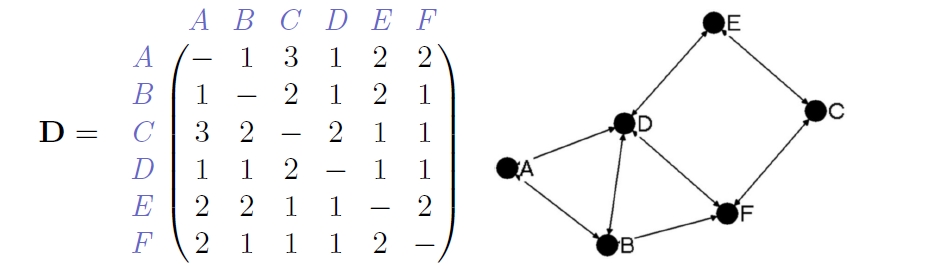
\(A\) - The adjacency matrix

\(P_{ij}\) - The expected connection between \(i\) and \(j\).

\(\lambda\) - Resolution parameter

Can use lots of different forms for \(P_{ij}\) but the standard one is the so called configuration model:

\(P_{ij} = \frac{k_i k_j}{2m}\)

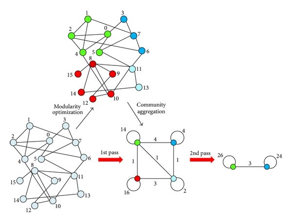
Loosely speaking, in an iterative process it

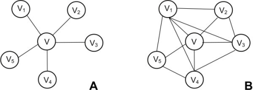
  1. You take a node and try to aggregate it to one of its neighbours.
  2. You choose the neighbour that maximizes a modularity function.
  3. Once you iterate through all the nodes, you will have merged few nodes together and formed some communities.
  4. This becomes the new input for the algorithm that will treat each community as a node and try to merge them together to create bigger communities.
  5. The algorithm stops when it’s not possible to improve modularity any more.

This is the original paper, for those interested in further reads:

  • Blondel, Vincent D; Guillaume, Jean-Loup; Lambiotte, Renaud; Lefebvre, Etienne (9 October 2008). “Fast unfolding of communities in large networks”. Journal of Statistical Mechanics: Theory and Experiment. 2008 (10): P10008

(Global) Network structure

(Global) Network structure

Finally, it is often also informative to look at the overal characteristics of the network. We will do this in more detail next time, but just so you know:

  • The density of a measure represents the share of all connected to all possible connections in the network
  • Transistivity, also called the Clustering Cefficient indicates how much the network tends to be locally clustered. That is measured by the share of closed triplets. Again,w e will dig into that next time.
  • The diameter is the longest of the shortest paths between two nodes of the network.
  • The mean distance, or average path lenght represents the mean of all shortest paths between all nodes. It is a measure of diffusion potential within a network.

Summing up

Summing up

In this session we talked about:

  1. What are networks and why might it be interesting to study them.
  2. What are commong datastructures to represent networks.
  3. What are basic definitions and concepts relevant for network analysis
  4. What are common measures of local network structure?
  5. What are common measures of global network structure?

Further readings

Textbooks

  • Jackson, Matthew O. Social and economic networks. Princeton university press, 2010.
  • Wasserman, Stanley, and Katherine Faust. Social network analysis: Methods and applications. Vol. 8. Cambridge university press, 1994.
  • Powell, Walter W., and Stine Grodal. “Networks of innovators.” Chapter in: The Oxford handbook of innovation” (2005).

Good research papers utulizing network analysis

  • Phelps, Corey, Ralph Heidl, and Anu Wadhwa. “Knowledge, networks, and knowledge networks: A review and research agenda.” Journal of management 38.4 (2012): 1115-1166.
  • Rakas, Marija, and Daniel S. Hain. “The state of innovation system research: What happens beneath the surface?.” Research Policy 48, no. 9 (2019): 103787.
  • Fleming, Lee, Charles King III, and Adam I. Juda. “Small worlds and regional innovation.” Organization Science 18.6 (2007): 938-954.
  • Hidalgo, César A., et al. “The product space conditions the development of nations.” Science 317.5837 (2007): 482-487.
  • Giuliani, Elisa, and Martin Bell. “The micro-determinants of meso-level learning and innovation: evidence from a Chilean wine cluster.” Research policy 34.1 (2005): 47-68.
  • Balland, Pierre-Alexandre, et al. “Smart specialization policy in the European Union: relatedness, knowledge complexity and regional diversification.” Regional Studies 53.9 (2019): 1252-1268.
  • Jurowetzki, Roman and Daniel S. Hain. Mapping the (r-) evolution of technological fields– a semantic network approach. In Luca M. Aiello and Dan McFarland, editors,SocialInformatics, volume 8851 ofLecture Notes in Computer Science, pages 359–383. Springer International Publishing, 2014.