Deconvolution and Image Segmentation
Group members: Johannes Hoseth, Sergiu Ropota, Katharina Granberg
Deconvolution - A Way Of Increasing Output Size
Within the field of computer vision, a well-known and multi-faceted area is segmentation, i.e. identifying and classifying objects in an image, via classes. Deep Learning is especially applicable for tackling this, since the models are effecient in finding higher-level indicative features used in the segmentation.
Convolutional Neural Networks (CNNs) are amongst the most used models for this, because they (a) work very resource-efficiently by basing their understanding locally, by scanning just a small area of the image at a time, using just enough weights. Conversely, a fully connected network scans the entire image, generating weights for each pixel.
We have chosen our topic to revolve around the lesser talked-about part of CNNs, being not the convolutional layers but rather the deconvolutional layers.
You'll find both some conceptual explanations alongside a concrete coding example, which we've made ourselves.
CNNs, In A Nutshell
CNNs consist basically of convolutional layers, where for each layer, a matrix-like filter is applied. The filter takes the dot product of all the pixel values underneath the filter and outputs the dot product as a singular value.
The addition of a pooling layer after the convolutional layer is common procedure used for ordering layers within a convolutional neural network and downsampling the image, making it smaller. Choosing a stride larger than 1 for the convolutional layer is another way of downsampling the image.
As this is done in multiple layers, the tensor becomes smaller and smaller, while its information becomes gradually more and more high-level. An example could be using CNN to recognizing cars in an image. The initial layers might recognize a car from low-level features that correspond to the vertical and horizontal lines of the boxy shape of a car. Later layers with more high-level features might be more complete representations of the car's symmetric shape, which combined with the lower-level features makes for an efficient holistic recognition process.

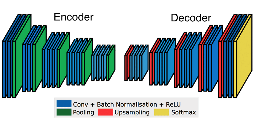
In the representation seen above, the general notion is that every convolutional layer is followed by the downsampling pooling layer. Before the pooling layer cna be applied, the ‘ReLu’ activation function is applied during convolution. The ReLu function goes through every pixel value and converts any negative value to zero. This effectively introduces non-lineraity into the model. Convolution is an otherwise linear operation, and since most of the real-world data is non-linear, the inclusion of ReLu accounts for that.
At the very end, a fully connected layer acts as the classifying function, basing its prediction on the high-level features acquired in the prior convolutional layers.
So What Does Deconvolution Do?
In image segmentation we don't just want to know which object is in the image, we want to know what kind of object each pixel in the image belongs to.
So for image segmentation the downsampled output poses a problem - we want to find the class of every pixel of the original image, so the outpus should be the original size of the image, and the downsampled output is not directly usable. We need to have an output image the same size as the input image. This is where deconvolution comes in!
Where regular convolutional layers encode features by downsampling, deconvolutional layers decodes that signal by upsampling. This means that it takes the minimized image and gradually increases its size back to its regular dimensions.
If one were in a hurry, the downsampled output image could just be randomly resized, but this looses information crucial for recognition. Instead, deconvolution is trainable (like regular convolution), with parameters/features free to change between the layers.
The way it does this is by taking a filter larger than the downsampled image, and by laying it over, multiplying the filter, the output becomes gradually bigger, as seen below:
This is the basic of deconvolution. We wanted to test it out ourselves and a set of images, so the reamining is a concrete coding example, of specifically deconvolution.
References:
‘A Beginner's guide to Deep Learning based Semantic Segmentation using Keras’ - https://divamgupta.com/image-segmentation/2019/06/06/deep-learning-semantic-segmentation-keras.html
‘Review: FCN — Fully Convolutional Network (Semantic Segmentation)’ - https://towardsdatascience.com/review-fcn-semantic-segmentation-eb8c9b50d2d1
‘Image Segmentation using deconvolution layer in Tensorflow’ - https://cv-tricks.com/image-segmentation/transpose-convolution-in-tensorflow/
‘A Gentle Introduction to Pooling Layers for Convolutional Neural Networks’ - https://machinelearningmastery.com/pooling-layers-for-convolutional-neural-networks/
‘Review: DeconvNet — Unpooling Layer (Semantic Segmentation)’ - https://towardsdatascience.com/review-deconvnet-unpooling-layer-semantic-segmentation-55cf8a6e380e
Coding example
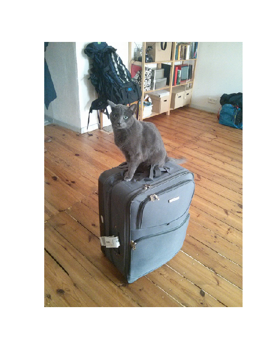
We got our data from the Common Objects in Context (COCO) database: http://cocodataset.org/#explore
They have images of common objects, with annotations on what objects are present in each picture an a mask highlighting each object.
Preample
%matplotlib inline
from pycocotools.coco import COCO
import numpy as np
import skimage.io as io
import matplotlib.pyplot as plt
import pylab
from PIL import Image
from IPython.display import Image as Img_open, display
pylab.rcParams['figure.figsize'] = (8.0, 10.0)
Data Handeling
First we create the folders we need in our directory, and then we download and unzip the data.
# Creating all the folders we need
!cd /content/; mkdir coco
!cd /content/coco/; mkdir images
!cd /content/coco/; mkdir annotations
!cd /content/coco/; mkdir imgs_train
!cd /content/coco/; mkdir imgs_test
!cd /content/coco/; mkdir masks
!cd /content/coco/; mkdir outputs
!wget http://images.cocodataset.org/zips/train2014.zip
!wget http://images.cocodataset.org/annotations/annotations_trainval2014.zip
#!wget http://images.cocodataset.org/annotations/image_info_test2014.zip
!unzip train2014.zip -d coco/images
!unzip annotations_trainval2014.zip -d coco/annotations/
We have chosen only to focus on regonising cats and dogs in images, so get a list of all the images containing cats and/or dogs.
# initialize COCO api for instance annotations
dataDir='coco'
dataType='train2014'
annFile='{}/annotations/annotations/instances_{}.json'.format(dataDir,dataType)
coco=COCO(annFile)
# Getting a list with the category IDs related to cats and dogs
catIds1 = coco.getCatIds(catNms=['cat'])
catIds2 = coco.getCatIds(catNms=['dog'])
catIds = catIds1+catIds2
# Getting a list with the image IDs for all images of cats and/or dogs
imgIds1 = coco.getImgIds(catIds=catIds1)
imgIds2 = coco.getImgIds(catIds=catIds2)
imgIds = list(set(imgIds1+imgIds2))
The first 1.000 images containing a cat/dog we use as our traning images.
First we save the images in a seperate folder that we call imgs_train, here we also rename them so the name is the image ID. Second we acess the mask for each image and save it in an other folder, that we call masks. It is important that they are named the same at their respective images. Third we recolor the masks, the model that we train later demand that the range of each image is only between 0 and 1.
import time
start = time.time()

# Preparing 1000 images and masks for training the model
for i in range(1000):       #len(imgIds) = 5715 images
  img=coco.loadImgs(imgIds[i])[0]
  I = io.imread(img['coco_url'])
  annIds = coco.getAnnIds(imgIds=img['id'], catIds=catIds, iscrowd=None)
  anns = coco.loadAnns(annIds)
  #Saving the image with no mask
  plt.imshow(I)
  plt.axis('off')
  plt.savefig('/content/coco/imgs_train/'+str(img['id'])+'.png')
  plt.close()
  #Saving the mask
  anns_img = np.zeros((img['height'],img['width']))
  anns_img = np.maximum(anns_img,coco.annToMask(anns[0])*anns[0]['category_id'])
  plt.imshow(anns_img, interpolation='nearest')
  plt.axis('off')
  plt.savefig('/content/coco/masks/'+str(img['id'])+'.png')
  plt.close()
  # # darkening the masks (making the pixels between 0 an 1)
  Image.open('/content/coco/masks/'+str(img['id'])+'.png').point(lambda p: p / 255).save('/content/coco/masks/'+str(img['id'])+'.png')
  # print(i) # just to follow the progress

end = time.time()
print(end - start)
552.9864583015442
We use the next 5 images containing a cat/dog as a test dataset.
# Preparing 5 images to test the model on
for i in range(1000,1005):
  img=coco.loadImgs(imgIds[i])[0]
  I = io.imread(img['coco_url'])
  annIds = coco.getAnnIds(imgIds=img['id'], catIds=catIds, iscrowd=None)
  anns = coco.loadAnns(annIds)
  #Saving the image with no mask
  plt.imshow(I)
  plt.axis('off')
  plt.savefig('/content/coco/imgs_test/'+str(img['id'])+'.png')
  plt.close()
The Model
We use a special package called keras-segmentation to create the model. It is a package made to work in tandem with Keras, so we use Keras functional API to describe the model.
Note the UpSampling2D layers, they are the ones doing the deconvolution.
# Importing the Keras modules
!pip install keras-segmentation
from keras_segmentation.models.model_utils import get_segmentation_model
from keras.layers import Input, Conv2D, Dropout, Conv2D, MaxPooling2D, UpSampling2D, concatenate
# Using the Keras functional API to define all the layers and the flow between them
img_input = Input(shape=(200, 200, 3 ))

conv1 = Conv2D(32, (3, 3), activation='relu', padding='same')(img_input)
conv1 = Dropout(0.2)(conv1)
conv1 = Conv2D(32, (3, 3), activation='relu', padding='same')(conv1)
pool1 = MaxPooling2D((2, 2))(conv1)

conv2 = Conv2D(64, (3, 3), activation='relu', padding='same')(pool1)
conv2 = Dropout(0.2)(conv2)
conv2 = Conv2D(64, (3, 3), activation='relu', padding='same')(conv2)
pool2 = MaxPooling2D((2, 2))(conv2)

conv3 = Conv2D(128, (3, 3), activation='relu', padding='same')(pool2)
conv3 = Dropout(0.2)(conv3)
conv3 = Conv2D(128, (3, 3), activation='relu', padding='same')(conv3)

up1 = concatenate([UpSampling2D((2, 2))(conv3), conv2], axis=-1)
conv4 = Conv2D(64, (3, 3), activation='relu', padding='same')(up1)
conv4 = Dropout(0.2)(conv4)
conv4 = Conv2D(64, (3, 3), activation='relu', padding='same')(conv4)

up2 = concatenate([UpSampling2D((2, 2))(conv4), conv1], axis=-1)
conv5 = Conv2D(32, (3, 3), activation='relu', padding='same')(up2)
conv5 = Dropout(0.2)(conv5)
conv5 = Conv2D(32, (3, 3), activation='relu', padding='same')(conv5)

out = Conv2D( 2, (1, 1) , padding='same')(conv5)
# Building the model as a segmentation model
model = get_segmentation_model(img_input ,  out )
Here we train the model, specifing the images and the masks to use.
# Training the model on the train images and their masks
model.train(
    train_images =  'coco/imgs_train',
    train_annotations = 'coco/masks',
    epochs = 2
)
Here we use the model to predict the appropriate mask highlighting cats and dogs in the image.
# Predict the mask for one image
out = model.predict_segmentation(
    inp='/content/coco/imgs_test/235062.png',
    out_fname='/content/coco/output.png'
)
display(Img_open('/content/coco/imgs_test/235062.png',width=100, height=100))
display(Img_open('/content/coco/output.png',width=100, height=100))

We found that the images that we use have a white frame outside them, because they are not all the same size, this is a problem we unfortunatly did not have time to solve. BUT we see how good the model is to predict a mask highlighting the frame! - even with just two epochs.
Here we make predictions for our 5 test images, and save them in the folder outputs.
# Predict masks for all the test images
model.predict_multiple(
	inp_dir='/content/coco/imgs_test/',
	out_dir='/content/coco/outputs/'
)
We do not have an intuitive understanding of the accuracy metric used by the segmentation_model so we have decided not to focus on this. Also since the frame has a way larger area than the cats/dogs on most of the images, it would probably just indicate how good it is at pedicting the frames.